Spooky Spectral Neural Networks (Part 1 of 2)
How Fourier Analysis Applies to Neural Networks

Overview
Neural networks are ubiquitous in modern machine learning owing to their powerful expressivity. If input data is drawn from some underlying equation of features, a neural network can quickly and robustly approximate that function. This approach is known as statistical learning and was the chief initial motivation for the development of neural networks in the 1990s.

However, there are limits to what classes of functions a neural network can learn. Expressivity is formally the size of the set of classes of functions that a neural network can fit. Expressivity is conditional on depth, layer activations, and network architecture among other things. Residual, convolutional, and recurrent neural networks all have very different classes of functions they can fit. For our purposes though, we will consider only the simple feed-forward neural network.

In this blog post, I’ll analyze the theoretical expressivity of a simple ReLU network, compare it to empirical results, and dive into a spectral perspective on expressivity. Fair warning: I am supposing some prior knowledge of neural networks in this post. If you need a reading reference, I recommend this guide.
A Walk in the “Latent Space” Park
A ReLU Network of size L is defined as a neural network with L hidden layers of varying dimensionality. The activation function for each of these layers is, of course, ReLU and the output layer at position L + 1 is a single output neuron. The behavior of the network can then be expressed as the following function.

The function T corresponds to the internals of a layer, which is defined by a weight matrix W and a bias b. Sigma is the activation function of ReLU. It is defined mathematically below.
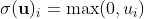
This activation function should look familiar and characteristic of the ReLU behavior. In this case, u is the feature vector and its entries are individual features.
This is how the layer function is defined. Now we have the preliminaries to describe a ReLU Network. The next thing we need is the definition of a Continuous Piecewise Linear Function (CPLF). The formal definition I’ll discuss next is a lot more involved, but we can achieve a quick and dirty intuitive understanding. A CPLF can be thought of as many different finite linear sections that are pasted together end to end into an infinite function.

The above function is an example of a CPLF in 2-dimensions. Formally, a CPLF is defined as follows.
“We say a function f: R^n → R is continuous piecewise linear if there exists a finite set of polyhedra whose union is R^n, and f is affine linear over each polyhedron (note that the definition automatically implies continuity of the function because the affine regions are closed and cover R^n, and affine functions are continuous).”
Whoa, interesting. What initially seemed intuitive suddenly involves sets of polyhedra and affine linearity. What happened there? Well, we can conceptualize our CPLF in n dimensions as the surface defined by a bunch of high-dimensional planes which intersect each other. Where these planes intersect, the resulting boundaries define a polyhedron. On these planes, we have affine linear space, which simply means the surface is flat and not curved, so moving in any direction behaves linearly.

It’s clear to see that any ReLU network represents a CPLF, considering the activation function is a CPLF in and of itself. It is less clear that any conceivable CPLF can be represented by a ReLU network. The proof is relatively simple to describe, though difficult to formalize.
Any CPLF can be described as a sum of a finite set of individual convex piecewise linear functions each of which can be described by a ReLU. It can also be shown that the sum of functions described by a ReLU network is also expressable by a ReLU network. It can then be shown that any CPLF can be expressed by a ReLU network of a certain depth as follows.
This universality is important. ReLU networks are essentially universal approximators. But how exactly does a ReLU network encode a CPLF? We can make it explicit mathematically.

In this case, P is a particular linear section of the CPLF referenced by the index epsilon and 1 is the indicator function for that linear section. Each linear section corresponds to an activation pattern of neurons in the hidden layers of the network. Along this linear section, certain neurons surpass the threshold of their activation function in a well-defined way. This phenomenon was explained eloquently in this paper.
Fourier Forays
We can now begin a Fourier analysis of ReLU networks or more specifically the CPLF represented by a ReLU network. Fourier analysis is a mathematical technique by which we break a function down into sine and cosine waves of varying amplitude and frequency, effectively mapping the function from time-space to frequency space. If you are unfamiliar with the technique, I recommend this paper.

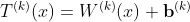
We can take the Fourier decomposition of piecewise linear functions similarly, although their lack of continuity leads to some interesting effects. For example, the Fourier decomposition of the simple piecewise function shown below is the sinc function.

Since our ReLU network is a CPLF and since that CPLF can be represented in the Fourier domain, we can effectively convert our neural network’s behavior into a frequency spectrum. We can compare how the frequency distribution of our network evolves as the neural network trains and see what information this reveals on the inner workings of our deep ReLU networks. Actually doing this decomposition takes a lot of math that isn’t super relevant for understanding intuition.
It’s a little easier to actually interpret the frequency. Remember, our goal was to use ReLU to approximate or express some other function black box that we can sample from. This function itself has a Fourier decomposition into bands of various frequencies. We can compare the Fourier spectrum of the function with that of our CPLF, and our hope is that training would cause these spectra to overlap.
The Grass Is Always Greener at Lower Frequency
It turns out that neural networks learn lower frequency trends first. This phenomenon is known as spectral bias. When tasked with approximating a complicated function, the first training steps in the ReLU network will fit the low-frequency components of that function. In the first experiment, we create a function to approximate by composing sinusoids of various frequencies and phases. Specifically, let k be the set of frequencies tested, A the set of corresponding amplitudes, and phi be the set of corresponding phases. The function to fit is then described as follows.

In the paper, the authors tested frequencies going from 5 to 50 hertz in increments of 5 and a randomized set of phases. In the first part, the amplitudes were constant and in the second part, the amplitudes increased as frequency increased. 200 points were sampled equally over the interval from 0 to 1 to constitute the training data for the ReLU network.
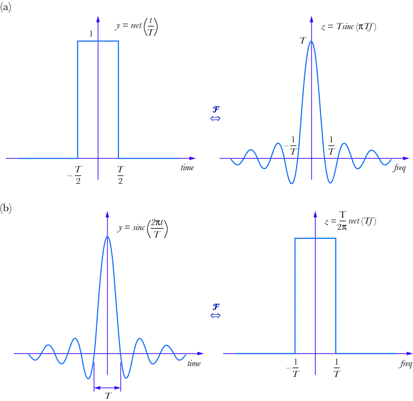
Here’s an example function generated by the first part. It’s a superposition of a lot of different sine waves, and the green sections represent what parts are learned by the ReLU network over the training cycle. At iteration 100, we have a very low-frequency sine wave that only loosely fits the data. At iteration 1,000, more high-frequency components are learned and it starts to loosely fit the spikes of the function. At iteration 10,000 the network accurately fits the start and end of the function including the high-frequency components, and after 80,000 cycles the function is well learned.
I enjoy this figure because it expresses visually what it means for a neural network to learn low-frequency trends. When pictured this way, it becomes apparent that ReLU networks are a learned patchwork of linear components which can be used to express complex trends.

This figure allows for a side-by-side comparison of part 1 and part 2. The “spectral norm of layer weights”, which is the y-axis of two of the figures, corresponds to the average frequency learned by the network. What’s fascinating is that even when low frequencies are many magnitudes higher in amplitude in the right figure, lower frequencies are still learned first. The spectral norm starts out low and only gradually increases.
The biggest difference between the two experiments is how the various layers learned frequencies. When amplitudes are equal, all of the layers learned roughly the same frequencies. However, when high-frequency sinusoids have a high amplitude, layers 2 and 5 seem to learn higher frequencies over the training cycles while layers 3 and 4 learn lower frequencies. It’s unclear why different layers specialize in different frequencies, or why this specialization seems arbitrary, and the question isn’t addressed in the original paper as well. Definitely a point of future investigation.
The second experiment demonstrates probably one of the most elegant ideas I’ve ever seen. The setup is very similar to the first experiment, and the authors allow the ReLU network to learn the target function to completion. In other words, the network has fully approximated the function with maximal accuracy. Then, they introduce a random perturbation of the ReLU net model weights and see how resilient the approximation is to change. The authors average and normalize over many random perturbations to understand how these perturbations impact the Fourier decomposition of the network.
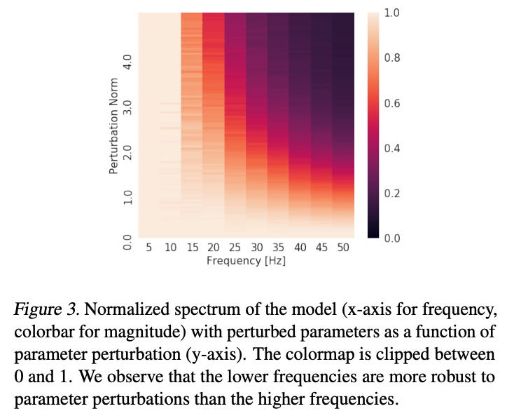
It turns out that lower frequencies are more resilient to perturbation. In other words, random changes to model weights destabilized high-frequency trends but had comparatively little effect on low-frequency trends. This suggests that in order to learn high-frequency trends, ReLU networks require careful calibration of weights across many layers which would also explain why they would learn these trends last.
There are other possible theoretical explanations for why this happens as well. Namely, the rate of change of the residual, or the error, decreases as the frequency of the fit increases. This disincentivizes fitting high-frequency trends as opposed to lower-frequency ones.
MNIST Strategist
MNIST is a benchmark dataset of images of handwritten numbers that’s been broadly cross-applied in assessing the performance of machine learning models. We can encode the 28x28 images into a 784-dimensional space in which our CPLF is defined. Since we’re now working with 784-dimensional functions instead of simple 1d functions, performing Fourier analysis on model training becomes way too hard. However, we have a few indirect ways to do this.
One way is that we can introduce perturbations to our images. Since we are now in 2-dimensional space, our perturbation takes the form of a radial wave which is like a sinusoidal spreading in all directions. We can test how high-frequency perturbation or noise as opposed to low-frequency noise impacts our model validation error, which is a surrogate for inverse model robustness.
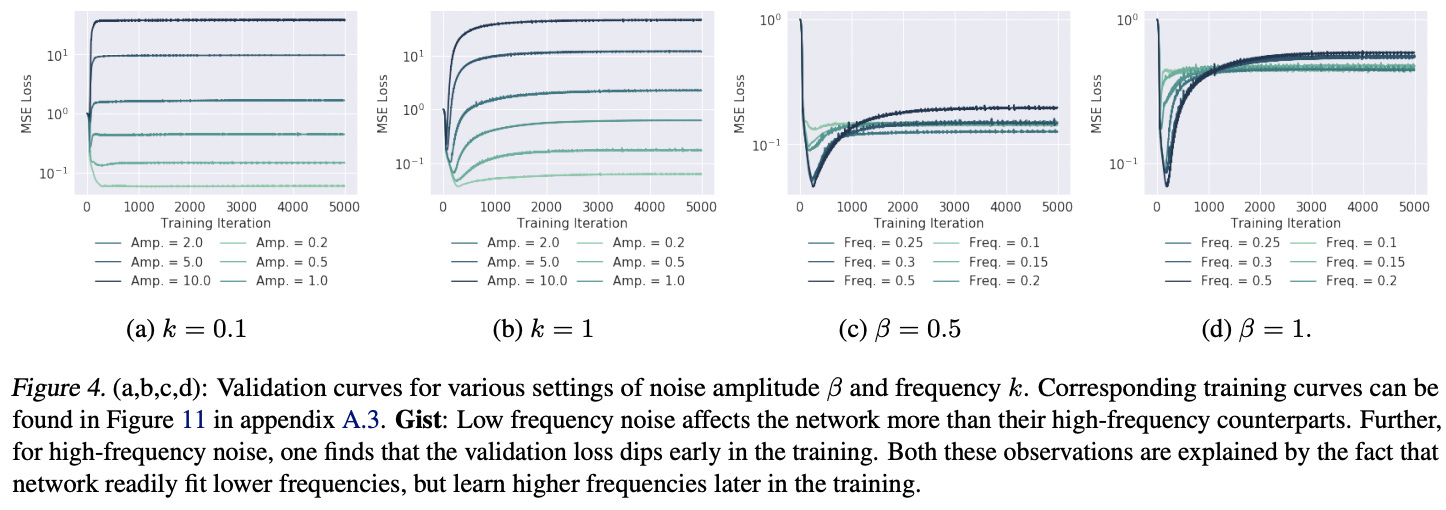
Perhaps unsurprisingly, low-frequency noise even at low amplitude has a positive impact on validation error (which means an inaccurate model). On the other hand, high-frequency radial noise does not significantly affect the model’s performance in the long term.
Exquisitely Eidetic Eigenfunctions
The most obvious next question is why we see the validation loss dip from high-frequency noise in the MNIST experiment above. To do this, we take an obvious and intuitive next step.
We simply project the CPLF encoded by the ReLU network to “the space spanned by the orthonormal eigenfunctions of the Gaussian radial basis function kernel”.
Easy enough, right? Let’s break it down.
An eigenfunction of a linear operator D is any function such that when D is applied to the function it is equivalent to multiplying the function by a scalar, which is the corresponding eigenvalue lambda.

In this case, the linear operator is the Gaussian radial basis function kernel, which is defined as follows between any two vectors x and y in our n-dimensional space. The function is also visualized in one dimension below.

 Kernel: The Go-To Kernel | by Sushanth Sreenivasa | Towards Data Science")
There are infinite possible eigenfunctions for this radial basis function since they extend in all directions. To define a span of our n-dimensional space, we just need an orthonormal subset of these eigenfunctions. In practice, these functions are similar to sinusoids in n-dimensional space.
We can use this definition to approximate the Fourier decomposition of the noise and ReLU network, which was previously too computationally expensive, as the decomposition in the space we have now spanned by our basis. When we do this, we get the following result.
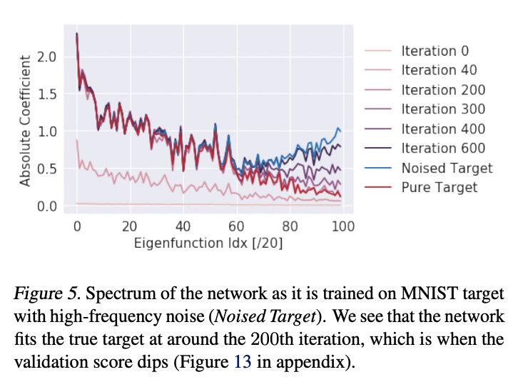
The higher eigenfunction index intuitively, but not rigorously, corresponds to a higher frequency. The validation loss decreases sharply around iteration 200, meaning our model becomes much more accurate because our model has learned the lower frequency actual data but not the higher frequency noise. As a result, in the figure, the iteration 200 performance fits the real target but not the noisy target. Over the next 400 cycles, however, the model learns the higher frequency noise causing its validation error to increase (since noise doesn’t carry over to validation).
What’s crazy is the implication of this for training neural networks. This essentially means it might be better to cut off training very early when faced with high-noise datasets. Your model will learn the low-frequency actual trends but not the high-frequency noise if spectral bias is handled efficiently.
Boo! The Article’s Over!
Spectral bias offers a different window into the inner workings of how neural networks learn trends. A Fourier perspective on ReLU networks could unveil so much more that we don’t know about how to optimize training, deal with noise, and improve expressivity. The authors make a point of encouraging future research in the field of Fourier analysis of neural networks, and for good reason. I’m positively spooked at the specter of all the possibilities!
In my next post, I’ll discuss the implications for learning manifolds which is the second part of the paper. My main goal with this sort of post is to take a groundbreaking paper that’s extremely technical but with a very high impact and decompose/synthesize it in a way that makes it accessible and understandable. I hope you enjoyed the post and stay tuned for a great first blog post from Eric sometime this week :)
Links:
Spectral bias and generalization
Acknowledgment
Most of the content discussed was derived originally from this paper. I would also like to thank Professor Hardt for explaining some of the concepts to me.