Using Overly High-Powered Models for Simple Problems (Part 2 of 3)
In this blog post series, we will be writing a Transformer model to solve the Repeated Prisoner's Dilemma problem.

Flashback
In my last post, I covered the basics of the repeated Prisoner’s Dilemma. In this post, I will formalize some of the mathematics behind the continuous Prisoner’s Dilemma and start writing some code.
Continuous Dilemma
Let’s assume we are an agent squaring off against the enemy agent based on the scenario provided in the last blog post. We have a notion of a reward matrix, which describes how much reward our agent gets based on what combination of actions the two agents choose. Let us set the value of 1 equal to defecting and 0 to cooperating. Here’s what our reward matrix then looks like:
# x indexing is our action, y indexing is opponent action
reward=[
    [3,0], # We cooperate
    [5,1]  # We defect
]
This is all good and fine until we realize that training a model on such a reward matrix and action space is impossible. This is because both are discrete, when our weights updating process (stochastic gradient descent) is fundamentally continuous. In other words, our model will almost surely fail to converge.
To solve this, we want to make both our action space and reward space continuous. For our action space, this is pretty easy. Instead of just having two choices (0 or 1), our agent can choose any real number between 0 and 1. However, it is unclear how to make our reward matrix continuous. We want our reward space to still be representative of our action space at the well-defined points. Let R(x, y) denote our reward function.
R(0,0)=3, R(0,1)=0, R(1,0)=5, R(1,1)=1To solve for the function R, we can perform a simple 2-dimensional linear interpolation. The formula for a 2d interpolation of our region is as follows.
f1 = 2x + 3
f2 = x
R(x,y) = [1-x, x] * reward.T * [[1-y],[y]]
F1 is the line defined by the reward at the two points where the opponent defects, (0,1) and (1,1). Similarly, F2 is the line defined by the reward at the two points where the opponent cooperates, (0,0) and (1,0). The resulting function can be defined by a simple matrix multiplication between an x matrix, the transpose of our reward matrix, and a y matrix.
In practice, we just use scipy’s 2d interpolation feature.
# Imports
import numpy as np
import scipy.interpolate as interpolate
import matplotlib.pyplot as plt

# X coords, y coords, and rewards respectively
x=[0,0,1,1]
y=[0,1,0,1]
z=[3,0,5,1]

# Perform interpolation
f=interpolate.interp2d(x,y,z,kind="linear")

# Apply to high-resolution discrete grid for visualization
new_x=np.linspace(0,1,1000)
new_y=np.linspace(0,1,1000)
result=f(new_x,new_y)

# Plot and format
fig, ax = plt.subplots()
plt.imshow(result,extent=[0,1,1,0])
plt.colorbar()
plt.gca().invert_yaxis()
plt.title("Continuous Interpolation of Reward")
ax.set_xlabel("Your Action")
ax.set_ylabel("Opponent Action")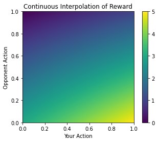
Looks pretty nice.
More importantly, it’s nice and continuous. There aren’t any obvious points where your model could get stuck and fail in its training process. If our agent outputted 0.5, then it would have a low-risk low reward sort of strategy, as we would expect. Thus, if it fails to learn the opponent's strategy we would expect it to output a lot of 0.5s.
It’s hard to explain our continuous reward intuitively. Let’s imagine the prisoner had instead of 1 bit of info, 2 bits of info. These 2 bits are mutually indistinguishable, so it is not as if bit 1 is informationally different from bit 2. Musk’s plan would go exceedingly well with both bits, but he can make somewhat do with 1 bit as well. Crucially, he doesn’t know there are 2 potential bits in play. You can cooperate and keep both bits safe, give up both bits and defect, OR you can give up just one bit and stay silent about the second bit. We can imagine taking the limit of the number of bits until we have an effectively infinite number of bits, and this is one way to conceptualize our reward.
The Environment
Let’s write a helper function.
def reward_func(my_action, opp_action):
  ans=np.matmul(np.array([1-my_action,my_action]),reward.T).reshape((1,2))
  return np.matmul(ans,np.array([[1-opp_action,opp_action]]).T).squeeze()
This function just calculates our reward. Now we can start writing some bots. Let’s start with the bots from the previous post.
import numpy as np

def CooperateRock(state_arr):
  return 1

def DefectRock(state_arr):
  return 0

def TitForTat(state_arr):
  # Check if array is empty
  if not np.any(state_arr):
    return 1
  if state_arr[1,-1] == 0:
    action = 0
  else:
    action = 1
  return action
Our agents take in a state array, of shape (4, num_games). The first row is our moves and the second row is the opponent’s moves. The third and fourth rows are the respective rewards of both parties. These bots are all discrete, but we can make some continuous bots too.
import random

def ModerateRock(state_arr):
  return 0.5

def RandomRock(state_arr):
  return random.random()

def AverageBot(state_arr, memory = None):
  if memory is None:
    memory=state_arr.shape[1]
  avg=np.mean(state_arr[1,-1*memory:])
  return avg
The last bot just plays the average of its opponent’s last memory actions. It can be considered a TitForTat bot if the memory is 1, for example. However, the memory can be longer and by default, the bot “remembers“ the entire history of how its opponent has played.
Datasets & Data Loaders
Since we have some bots, we can start generating datasets for our transformer model.
class p_dataset(data.Dataset, ABC):
  def __init__(self, agents, reward, runs=1000):
    self.agents=agents
    self.reward=reward
    self.state_arr=np.zeros((4,1))

  def __len__(self):
    return self.state_arr.shape[1]-1

  # Return the first n games, and the result of game n+1
  # Constitutes the input and label data respectively
  def __getitem__(self, idx):
    return self.state_arr[:,:idx], self.state_arr[:2,idx+1].squeeze()

  def __repr__(self):
    return np.array2string(self.state_arr)

  def reward_func(self,my_action, opp_action, reward_mat):
    ans=np.matmul(np.array([1-my_action,my_action]), reward_mat.T)
    return np.matmul(ans.reshape((1,2)),np.array([[1-opp_action,opp_action]]).T).squeeze()

  def simulate(self, n_sims=100):
    for i in range(n_sims):
      moves=self.state_arr

      # Compute agent actions
      action1=self.agents[0](self.state_arr)
      action2=self.agents[1](np.flip(self.state_arr, axis=0))
      rew1=self.reward_func(action1, action2, self.reward) # Compute rewards
      rew2=self.reward_func(action2, action1, self.reward)

      # Add to state tensor
      self.state_arr = np.append(self.state_arr, np.array([action1, action2,rew1,rew2]).reshape((4,1)),axis=1)
We now have a very basic PyTorch dataset class. It stores the outcomes of a continued set of matches between two agents. We can simulate as many matches as we want and use this dataset to train our models. Let’s test it by playing AverageBot against RandomRock.
from torch.utils.data import DataLoader

# Initialize dataset
training_data=p_dataset([AverageBot, RandomRock],reward)
test_data=p_dataset([AverageBot, RandomRock],reward)

# Run simulations
training_data.simulate()
test_data.simulate(n_sims=40)

# Initialize dataloaders
train_dataloader = DataLoader(training_data, batch_size=16, shuffle=True)
test_dataloader = DataLoader(test_data, batch_size=16, shuffle=True)
Let’s look at our simulation data and see if it makes sense.
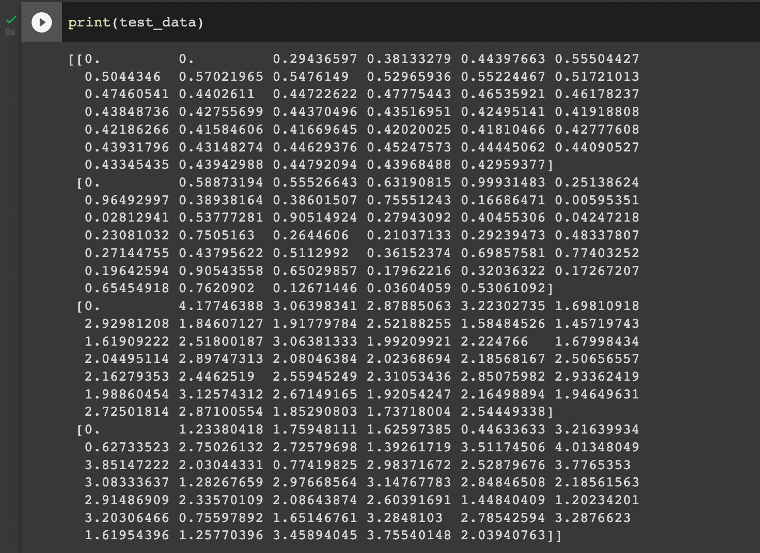
How do we interpret this output? Remember our state array consists of four subarrays. The first subarray, which is the topmost, is AverageBot’s actions. The second subarray, which is second from the top, is RandomRock’s actions. In the first two games, AverageBot plays 0, since the average of the last few moves of Random Rock is also 0. On the third round, AverageBot sees RandomRock’s history of playing 0 then 0.588, and correctly plays the average of 0.294. The third and fourth arrays are the reward for AverageBot and RandomRock respectively.
Looks like our random bot is doing random things, and our average bot is mirroring the average output over random bot’s history (which effectively means it also does random things). Awesome!
Total score over n=40 games for average bot: 94.9475094
Total score over n=40 games for random bot: 94.4639304
AverageBot is winning by a very slim margin, which we would hope to see considering it’s somewhat smarter than its opponent, RandomRock.
What’s To Come
Now that we have a PyTorch training & test data loader, all that’s left is to use them to train/test our Transformer model to predict how bots will play! In my next post, I’ll introduce the Transformer architecture and write a basic model in PyTorch. I’ll train it to predict the prisoner’s dilemma and (hopefully) get some good results. Until next time!